Discontinuous Molecular Dynamics
Discontinuous Molecular Dynamics (DMD) is a special method of coarse graining an available potential field in which a continuous potential is approximated by step and shoulder potentials and is then used for performing molecular dynamics simulations. Depending on the length and timescale of the problem being considered, it is possible to apply DMD to many continuous potential fields by discretizing them into multiple square well or shoulder potentials.
The first application of this method to peptides was presented in early 2000s [13-15]. They parameterized the various interactions between molecules in a polymer chain (including alkanes, peptides and proteins) such as bond movements, angle changes and chain movements as a whole. For peptides, they developed a new force field which can be used in DMD simulations, dubbed PRIME20 (for the 20 natural amino acids). Using the PRIME20 forcefield, they were able to study the formation of secondary and tertiary structures in peptides, analyze their folding mechanism, and determine stable structures corresponding to different external conditions. In recent years, PRIME20 and DMD have been used to identify molecules and conformations that can help stop or restrict depreciatory biologically active molecules such as prion proteins and glaucoma causing amyloid molecules.DMD has previously been applied to a wide variety of biomolecular systems. In this section, we will focus on their application to peptides, which are the molecules closest to our system of interest: the peptoids. One of the early papers to discuss molecular dynamics [8] described the dynamics of square well particles. After this, through various applications in chain dynamics by Rapaport [9], the method was ready to be used in chain molecules. The challenge of improving the efficiency of this method was then taken up by Smith et.al. [10], where they explain in detail features such as timelists, neighbor lists and scheduling of events to increase the speed of the simulation method for polymer chains. Using DMD for polymers, Hall and her group at NCSU were able to analyze various properties of long-chain molecules such as the effect of chain rigidity on phase transitions as well as the relationship between chain branching and phase transitions.
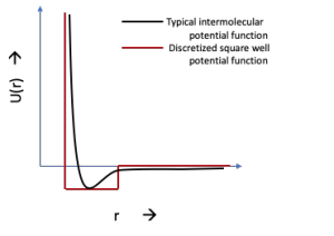
Discretized form of a continuous potential which used in a DMD simulation
They and other groups [11,12] have used discretized all-atom potentials to develop the corresponding square well potentials for DMD applications. Our proposed method will be based on the general methodology of PRIME20, but with the modifications needed for simulating peptoids.
One of the limitations of DMD is that so far, it has been used in single processor codes. In recent years, there have been some efforts to use parallel architectures for simulating DMD systems [16,17]. These approaches, though being a much-needed first step, still keep the nodes that are performing successive moves idle for a long time. Furthermore, there is no sure-fire way to ensure that the data generated will be incorporated in the running list at the main node, as those events might, at the end, be canceled due to other intermediate collisions. Therefore, there is a need to eliminate these limitations of DMD as well.
A general DMD force field
The major challenge in any general force field is finding the parameters for a multitude of forces. A simple example of the force field can be the one described below:

The various potential components between molecules are as follows: bond energy between two molecules (force constant K1, equilibrium bond length b0), Urey-Bradley potential (force constant KUB, equilibrium Urey-Bradley term S0), bond angle potentials modeled as springs (force constant Kθ, equilibrium angle θ0 ), dihedral angle potentials (force constant Kχ , dihedral multiplicity n and phase d), improper angle potentials with force constant Kimp and the equilibrium potential as f0 and nonbonded parameters, which include electrostatic interactions (with q being the charge on the interacting particles, rij being the distance between them and e1 as the dielectric constant of the medium) and Lennard Jones potentials accounting for dispersion and overlap forces (with Rmin as the 6-12 Lennard Jones (LJ) radius and e as the LJ potential well depth ). Using a continuous potential has the disadvantage that we have to follow Newton’s laws of motion and move the particles by a fixed timestep to ensure stability and to keep the approximations in the potentials to a manageable degree (which increase as a power of the timestep), which swell a lot in the case of an improper timestep. Studying a typical molecule at this scale, the fastest degree of freedom are bond vibrations, moving with an approximate timestep of 10 femtosecond (fs). In a good molecular dynamics simulation, the timestep should be less than 10% of the time for the smallest motion, which in this case becomes 1 fs, which is too short a timestep to go to a real-life timescale. To overcome this issue, as well as to increase the speed of the simulations, a suitable approximation is to estimate each of the potential as a square well (Figure 2b), which, usually, is given by
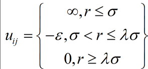
A separate potential well is generated for each of the many different types of potentials mentioned above, with a different well depth e, hard-sphere radius s and square well cutoff ls.
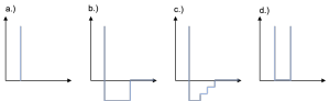
Graphical representations of a.) Hard sphere potential b.) Square Well potential c.) Square well potential with multiple levels d.) Infinite square well bonding potentials. X-axis: Distance between two particles and Y-axis: Potential value
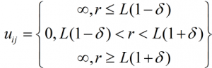
Therefore, the major challenge in perfecting a parameterised DMD field is to find these parameters that can generate results similar to those obtained by atomistic simulations or experimental analysis. Furthermore, an interesting method introduced by Rapaport [9] was to use discontinuous potentials to model bonds (Figure 5d). Any bond was allowed to change its length by a small number “2δ”, so, if the bond length initially was ‘L’, then the bond length could fluctuate between L(1+ δ) and L(1- δ), which makes it a square potential well with zero well depth, as given by
DMD force fields for peptides have proven to be anywhere between 3-10 times faster than the average molecular dynamics simulations [24-26]. An important reason for this can be that for less dense systems, moving particles by a fixed, small timestep (as in MD) consumes valuable computational time, which can be bypassed when we use DMD. At high densities, both MD and DMD simulations might be expected to take similar time, but the simplification in calculations required when using a square-well type potential field make DMD simulations run faster even for dense systems. For initially configuring the particles, the velocities are usually initialized with a Maxwell-Boltzmann distribution congruent with the temperature at which the system is being studied. The positions are random inside the simulation box, but care must be taken that the bond parameters such as length and angle constraints are not violated. The general algorithm is shown in Figure 3.
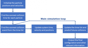
A typical Discontinuous Molecular Dynamics algorithm